Kernel Marginal Fisher Analysis (KMFA) is a nonlinear variant of MFA using kernel tricks. For simplicity, we only enabled a heat kernel of a form $$k(x_i,x_j)=\exp(-d(x_i,x_j)^2/2*t^2)$$ where \(t\) is a bandwidth parameter. Note that the method is far sensitive to the choice of \(t\).
Arguments
- X
an \((n\times p)\) matrix or data frame whose rows are observations.
- label
a length-\(n\) vector of data class labels.
- ndim
an integer-valued target dimension.
- preprocess
an additional option for preprocessing the data. Default is "center". See also
aux.preprocessfor more details.- k1
the number of same-class neighboring points (homogeneous neighbors).
- k2
the number of different-class neighboring points (heterogeneous neighbors).
- t
bandwidth parameter for heat kernel in \((0,\infty)\).
Value
a named list containing
- Y
an \((n\times ndim)\) matrix whose rows are embedded observations.
- trfinfo
a list containing information for out-of-sample prediction.
References
Yan S, Xu D, Zhang B, Zhang H, Yang Q, Lin S (2007). “Graph Embedding and Extensions: A General Framework for Dimensionality Reduction.” IEEE Transactions on Pattern Analysis and Machine Intelligence, 29(1), 40–51.
Examples
## generate data of 3 types with clear difference
set.seed(100)
dt1 = aux.gensamples(n=20)-100
dt2 = aux.gensamples(n=20)
dt3 = aux.gensamples(n=20)+100
## merge the data and create a label correspondingly
X = rbind(dt1,dt2,dt3)
label = rep(1:3, each=20)
## try different numbers for neighborhood size
out1 = do.kmfa(X, label, k1=10, k2=10, t=0.001)
out2 = do.kmfa(X, label, k1=10, k2=10, t=0.01)
out3 = do.kmfa(X, label, k1=10, k2=10, t=0.1)
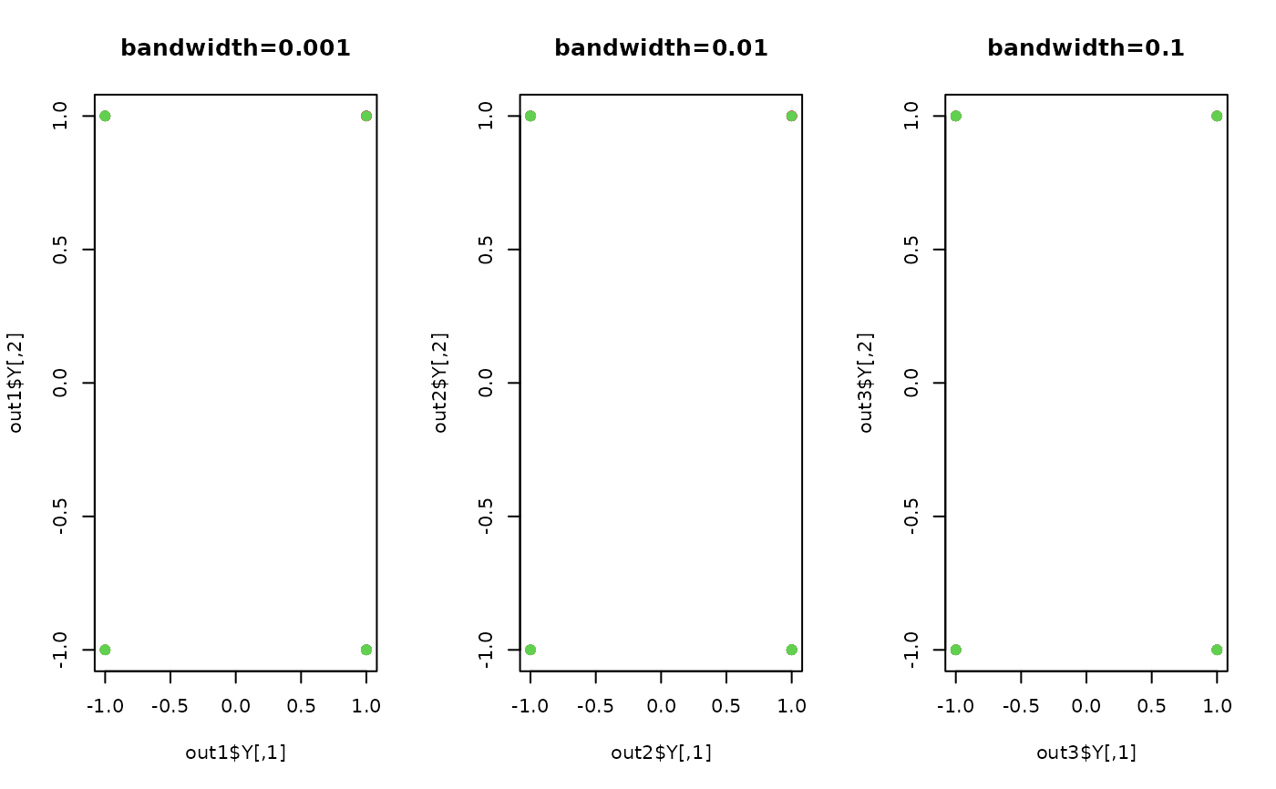
## visualize
opar = par(no.readonly=TRUE)
par(mfrow=c(1,3))
plot(out1$Y, pch=19, col=label, main="bandwidth=0.001")
plot(out2$Y, pch=19, col=label, main="bandwidth=0.01")
plot(out3$Y, pch=19, col=label, main="bandwidth=0.1")
 par(opar)