Many variants of Locality Preserving Projection are contingent on graph construction schemes in that they sometimes return a range of heterogeneous results when parameters are controlled to cover a wide range of values. This algorithm takes an approach called sample-dependent construction of graph connectivity in that it tries to discover intrinsic structures of data solely based on data.
do.sdlpp(
  X,
  ndim = 2,
  t = 1,
  preprocess = c("center", "scale", "cscale", "decorrelate", "whiten")
)
Arguments
- X
an \((n\times p)\) matrix or data frame whose rows are observations.
- ndim
an integer-valued target dimension.
- t
kernel bandwidth in \((0,\infty)\).
- preprocess
an additional option for preprocessing the data. Default is "center". See also
aux.preprocessfor more details.
Value
a named list containing
- Y
an \((n\times ndim)\) matrix whose rows are embedded observations.
- trfinfo
a list containing information for out-of-sample prediction.
- projection
a \((p\times ndim)\) whose columns are basis for projection.
References
Yang B, Chen S (2010). “Sample-Dependent Graph Construction with Application to Dimensionality Reduction.” Neurocomputing, 74(1-3), 301--314.
See also
Examples
## use iris data
data(iris)
set.seed(100)
subid = sample(1:150, 50)
X = as.matrix(iris[subid,1:4])
label = as.factor(iris[subid,5])
## compare with PCA
out1 <- do.pca(X,ndim=2)
out2 <- do.sdlpp(X, t=0.01)
out3 <- do.sdlpp(X, t=10)
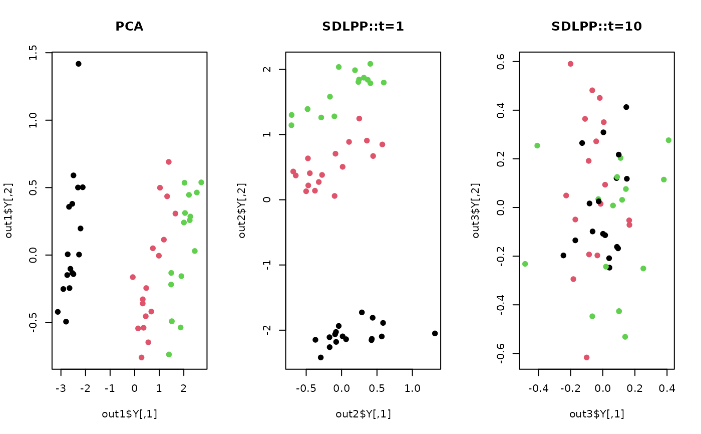
## visualize
opar <- par(no.readonly=TRUE)
par(mfrow=c(1,3))
plot(out1$Y, pch=19, col=label, main="PCA")
plot(out2$Y, pch=19, col=label, main="SDLPP::t=1")
plot(out3$Y, pch=19, col=label, main="SDLPP::t=10")
 par(opar)