This function robustifies the traditional PCA via an idea of geometric median.
To describe, the given data is first split into k subsets for each sample
covariance is attained. According to the paper, the median covariance is computed
under Frobenius norm and projection is extracted from the largest eigenvectors.
do.rpcag(
  X,
  ndim = 2,
  k = 5,
  preprocess = c("center", "scale", "cscale", "whiten", "decorrelate")
)
Arguments
- X
an \((n\times p)\) matrix or data frame whose rows are observations and columns represent independent variables.
- ndim
an integer-valued target dimension.
- k
the number of subsets for
Xto be divided.- preprocess
an additional option for preprocessing the data. Default is "center". See also
aux.preprocessfor more details.
Value
a named list containing
- Y
an \((n\times ndim)\) matrix whose rows are embedded observations.
- trfinfo
a list containing information for out-of-sample prediction.
- projection
a \((p\times ndim)\) whose columns are basis for projection.
References
Minsker S (2015). “Geometric Median and Robust Estimation in Banach Spaces.” Bernoulli, 21(4), 2308--2335.
Examples
## use iris data
data(iris)
X     = as.matrix(iris[,1:4])
label = as.integer(iris$Species)

## try different numbers for subsets
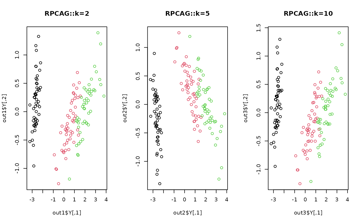
out1 = do.rpcag(X, ndim=2, k=2)
out2 = do.rpcag(X, ndim=2, k=5)
out3 = do.rpcag(X, ndim=2, k=10)

## visualize
opar <- par(no.readonly=TRUE)
par(mfrow=c(1,3))
plot(out1$Y, col=label, main="RPCAG::k=2")
plot(out2$Y, col=label, main="RPCAG::k=5")
plot(out3$Y, col=label, main="RPCAG::k=10")

par(opar)