Random Projection — do.rndproj • Rdimtools

do.rndproj is a linear dimensionality reduction method based on random projection technique, featured by the celebrated Johnson–Lindenstrauss lemma.

do.rndproj(
  X,
  ndim = 2,
  preprocess = c("null", "center", "scale", "cscale", "whiten", "decorrelate"),
  type = c("gaussian", "achlioptas", "sparse"),
  s = max(sqrt(ncol(X)), 3)
)

Arguments

X: an $(n\times p)$ matrix or data frame whose rows are observations and columns represent independent variables.
ndim: an integer-valued target dimension.
preprocess: an additional option for preprocessing the data. Default is "null". See also aux.preprocess for more details.
type: a type of random projection, one of "gaussian","achlioptas" or "sparse".
s: a tuning parameter for determining values in projection matrix. While default is to use $max(log \sqrt{p},3)$ , it is required for $s \ge 3$ .

Value

a named list containing

Y: an $(n\times ndim)$ matrix whose rows are embedded observations.
projection: a $(p\times ndim)$ whose columns are basis for projection.
epsilon: an estimated error $\epsilon$ in accordance with JL lemma.
trfinfo: a list containing information for out-of-sample prediction.

Details

The Johnson-Lindenstrauss(JL) lemma states that given $0 < \epsilon < 1$ , for a set $X$ of $m$ points in $R^N$ and a number $n > 8log(m)/\epsilon^2$ , there is a linear map $f:R^N$ to R^n such that $(1-\epsilon)|u-v|^2 \le |f(u)-f(v)|^2 \le (1+\epsilon)|u-v|^2$ for all $u,v$ in $X$ .

Three types of random projections are supported for an (p-by-ndim) projection matrix $R$ .

Conventional approach is to use normalized Gaussian random vectors sampled from unit sphere $S^{p-1}$ .
Achlioptas suggested to employ a sparse approach using samples from $\sqrt{3}(1,0,-1)$ with probability $(1/6,4/6,1/6)$ .
Li et al proposed to sample from $\sqrt{s}(1,0,-1)$ with probability $(1/2s,1-1/s,1/2s)$ for $s\ge 3$ to incorporate sparsity while attaining speedup with little loss in accuracy. While the original suggsetion from the authors is to use $\sqrt{p}$ or $p/log(p)$ for $s$ , any user-supported $s \ge 3$ is allowed.

References

Johnson WB, Lindenstrauss J (1984). “Extensions of Lipschitz Mappings into a Hilbert Space.” In Beals R, Beck A, Bellow A, Hajian A (eds.), Contemporary Mathematics, volume 26, 189--206. American Mathematical Society, Providence, Rhode Island. ISBN 978-0-8218-5030-5 978-0-8218-7611-4.

Achlioptas D (2003). “Database-Friendly Random Projections: Johnson-Lindenstrauss with Binary Coins.” Journal of Computer and System Sciences, 66(4), 671--687.

Li P, Hastie TJ, Church KW (2006). “Very Sparse Random Projections.” In Proceedings of the 12th ACM SIGKDD International Conference on Knowledge Discovery and Data Mining, KDD '06, 287--296.

Examples

## use iris data
data(iris)
set.seed(100)
subid = sample(1:150, 50)
X     = as.matrix(iris[subid,1:4])
label = as.factor(iris[subid,5])

## 1. Gaussian projection
output1 <- do.rndproj(X,ndim=2)

## 2. Achlioptas projection
output2 <- do.rndproj(X,ndim=2,type="achlioptas")

## 3. Sparse projection
output3 <- do.rndproj(X,type="sparse")

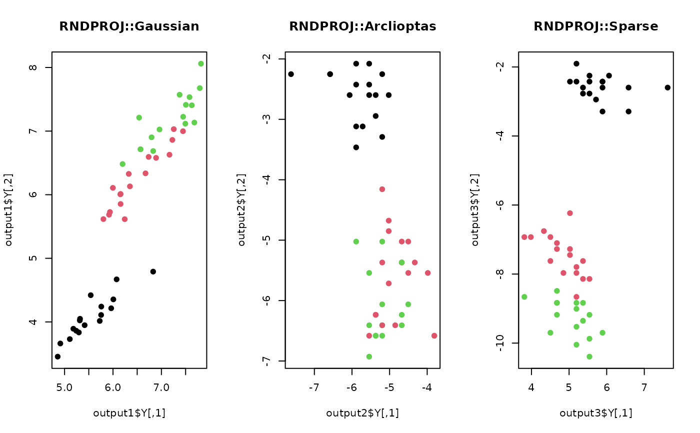
## Visualize three different projections
opar <- par(no.readonly=TRUE)
par(mfrow=c(1,3))
plot(output1$Y, pch=19, col=label, main="RNDPROJ::Gaussian")
plot(output2$Y, pch=19, col=label, main="RNDPROJ::Arclioptas")
plot(output3$Y, pch=19, col=label, main="RNDPROJ::Sparse")

par(opar)