Landmark MDS is a variant of Classical Multidimensional Scaling in that it first finds a low-dimensional embedding using a small portion of given dataset and graft the others in a manner to preserve as much pairwise distance from all the other data points to landmark points as possible.
Arguments
- X
an \((n\times p)\) matrix whose rows are observations and columns represent independent variables.
- ndim
an integer-valued target dimension.
- npoints
the number of landmark points to be drawn.
Value
a named Rdimtools S3 object containing
- Y
an \((n\times ndim)\) matrix whose rows are embedded observations.
- projection
a \((p\times ndim)\) whose columns are basis for projection.
- algorithm
name of the algorithm.
References
Silva VD, Tenenbaum JB (2002). “Global Versus Local Methods in Nonlinear Dimensionality Reduction.” In Thrun S, Obermayer K (eds.), Advances in Neural Information Processing Systems 15, 705--712. MIT Press, Cambridge, MA.
Lee S, Choi S (2009). “Landmark MDS Ensemble.” Pattern Recognition, 42(9), 2045--2053.
See also
Examples
# \donttest{
## use iris data
data(iris)
X = as.matrix(iris[,1:4])
lab = as.factor(iris[,5])
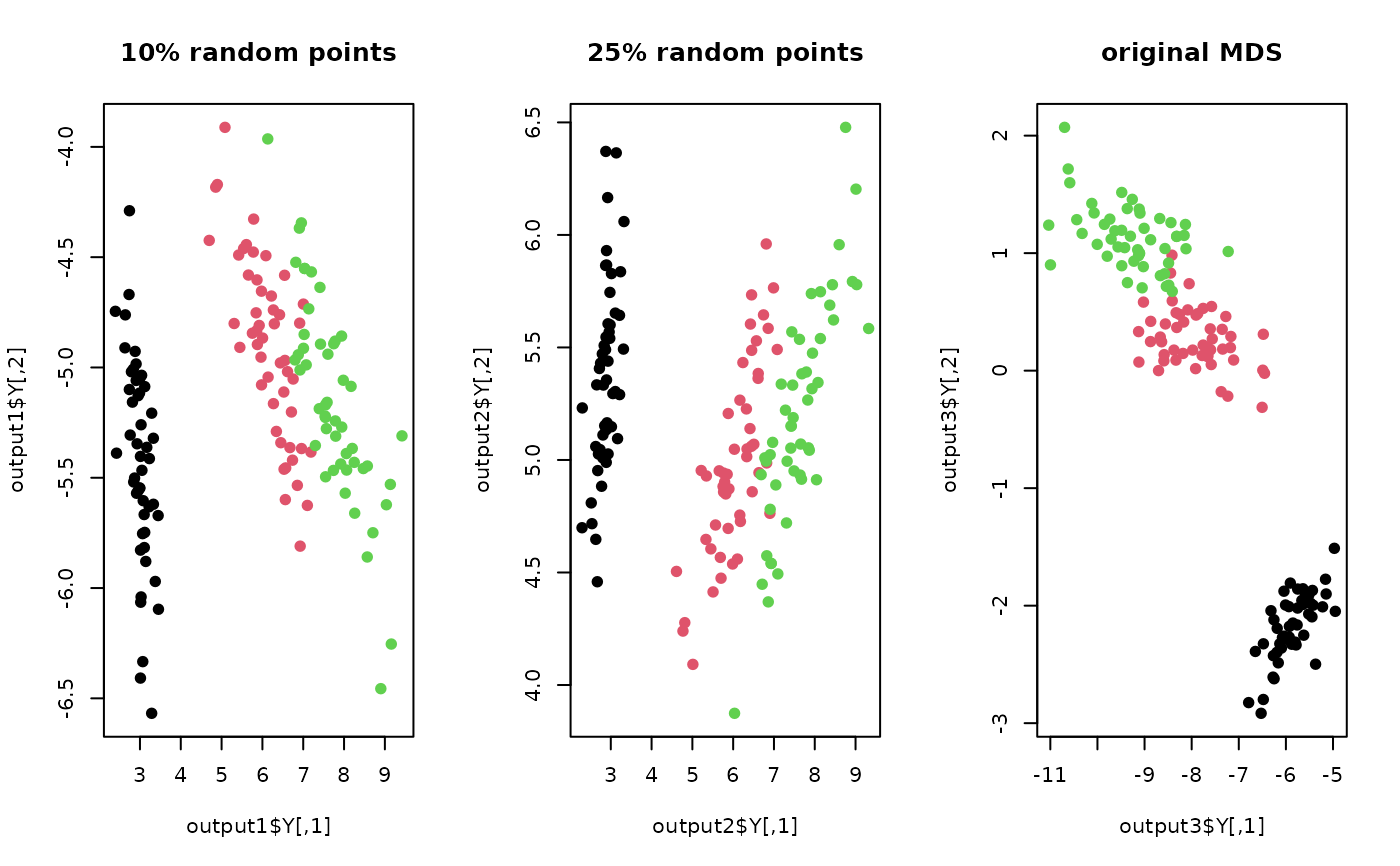
## use 10% and 25% of the data and compare with full MDS
output1 <- do.lmds(X, ndim=2, npoints=round(nrow(X)*0.10))
output2 <- do.lmds(X, ndim=2, npoints=round(nrow(X)*0.25))
output3 <- do.mds(X, ndim=2)
## vsualization
opar <- par(no.readonly=TRUE)
par(mfrow=c(1,3))
plot(output1$Y, pch=19, col=lab, main="10% random points")
plot(output2$Y, pch=19, col=lab, main="25% random points")
plot(output3$Y, pch=19, col=lab, main="original MDS")
 par(opar)
# }
par(opar)
# }