From the celebrated Mercer's Theorem, we know that for a mapping \(\phi\), there exists
a kernel function - or, symmetric bilinear form, \(K\) such that $$K(x,y) = <\phi(x),\phi(y)>$$ where \(<,>\) is
standard inner product. aux.kernelcov is a collection of 20 such positive definite kernel functions, as
well as centering of such kernel since covariance requires a mean to be subtracted and
a set of transformed values \(\phi(x_i),i=1,2,\dots,n\) are not centered after transformation.
Since some kernels require parameters - up to 2, its usage will be listed in arguments section.
aux.kernelcov(X, ktype)Arguments
- X
an \((n\times p)\) data matrix
- ktype
a vector containing the type of kernel and parameters involved. Below the usage is consistent with description
- linear
c("linear",c)- polynomial
c("polynomial",c,d)- gaussian
c("gaussian",c)- laplacian
c("laplacian",c)- anova
c("anova",c,d)- sigmoid
c("sigmoid",a,b)- rational quadratic
c("rq",c)- multiquadric
c("mq",c)- inverse quadric
c("iq",c)- inverse multiquadric
c("imq",c)- circular
c("circular",c)- spherical
c("spherical",c)- power/triangular
c("power",d)- log
c("log",d)- spline
c("spline")- Cauchy
c("cauchy",c)- Chi-squared
c("chisq")- histogram intersection
c("histintx")- generalized histogram intersection
c("ghistintx",c,d)- generalized Student-t
c("t",d)
Value
a named list containing
- K
a \((p\times p)\) kernelizd gram matrix.
- Kcenter
a \((p\times p)\) centered version of
K.
Details
There are 20 kernels supported. Belows are the kernels when given two vectors \(x,y\), \(K(x,y)\)
- linear
\(=<x,y>+c\)
- polynomial
\(=(<x,y>+c)^d\)
- gaussian
\(=exp(-c\|x-y\|^2)\), \(c>0\)
- laplacian
\(=exp(-c\|x-y\|)\), \(c>0\)
- anova
\(=\sum_k exp(-c(x_k-y_k)^2)^d\), \(c>0,d\ge 1\)
- sigmoid
\(=tanh(a<x,y>+b)\)
- rational quadratic
\(=1-(\|x-y\|^2)/(\|x-y\|^2+c)\)
- multiquadric
\(=\sqrt{\|x-y\|^2 + c^2}\)
- inverse quadric
\(=1/(\|x-y\|^2+c^2)\)
- inverse multiquadric
\(=1/\sqrt{\|x-y\|^2+c^2}\)
- circular
\(= \frac{2}{\pi} arccos(-\frac{\|x-y\|}{c}) - \frac{2}{\pi} \frac{\|x-y\|}{c}\sqrt{1-(\|x-y\|/c)^2} \), \(c>0\)
- spherical
\(= 1-1.5\frac{\|x-y\|}{c}+0.5(\|x-y\|/c)^3 \), \(c>0\)
- power/triangular
\(=-\|x-y\|^d\), \(d\ge 1\)
- log
\(=-\log (\|x-y\|^d+1)\)
- spline
\(= \prod_i ( 1+x_i y_i(1+min(x_i,y_i)) - \frac{x_i + y_i}{2} min(x_i,y_i)^2 + \frac{min(x_i,y_i)^3}{3} ) \)
- Cauchy
\(=\frac{c^2}{c^2+\|x-y\|^2}\)
- Chi-squared
\(=\sum_i \frac{2x_i y_i}{x_i+y_i}\)
- histogram intersection
\(=\sum_i min(x_i,y_i)\)
- generalized histogram intersection
\(=sum_i min( |x_i|^c,|y_i|^d )\)
- generalized Student-t
\(=1/(1+\|x-y\|^d)\), \(d\ge 1\)
References
Hofmann, T., Scholkopf, B., and Smola, A.J. (2008) Kernel methods in machine learning. arXiv:math/0701907.
Examples
# \donttest{
## generate a toy data
set.seed(100)
X = aux.gensamples(n=100)
## compute a few kernels
Klin = aux.kernelcov(X, ktype=c("linear",0))
Kgau = aux.kernelcov(X, ktype=c("gaussian",1))
Klap = aux.kernelcov(X, ktype=c("laplacian",1))
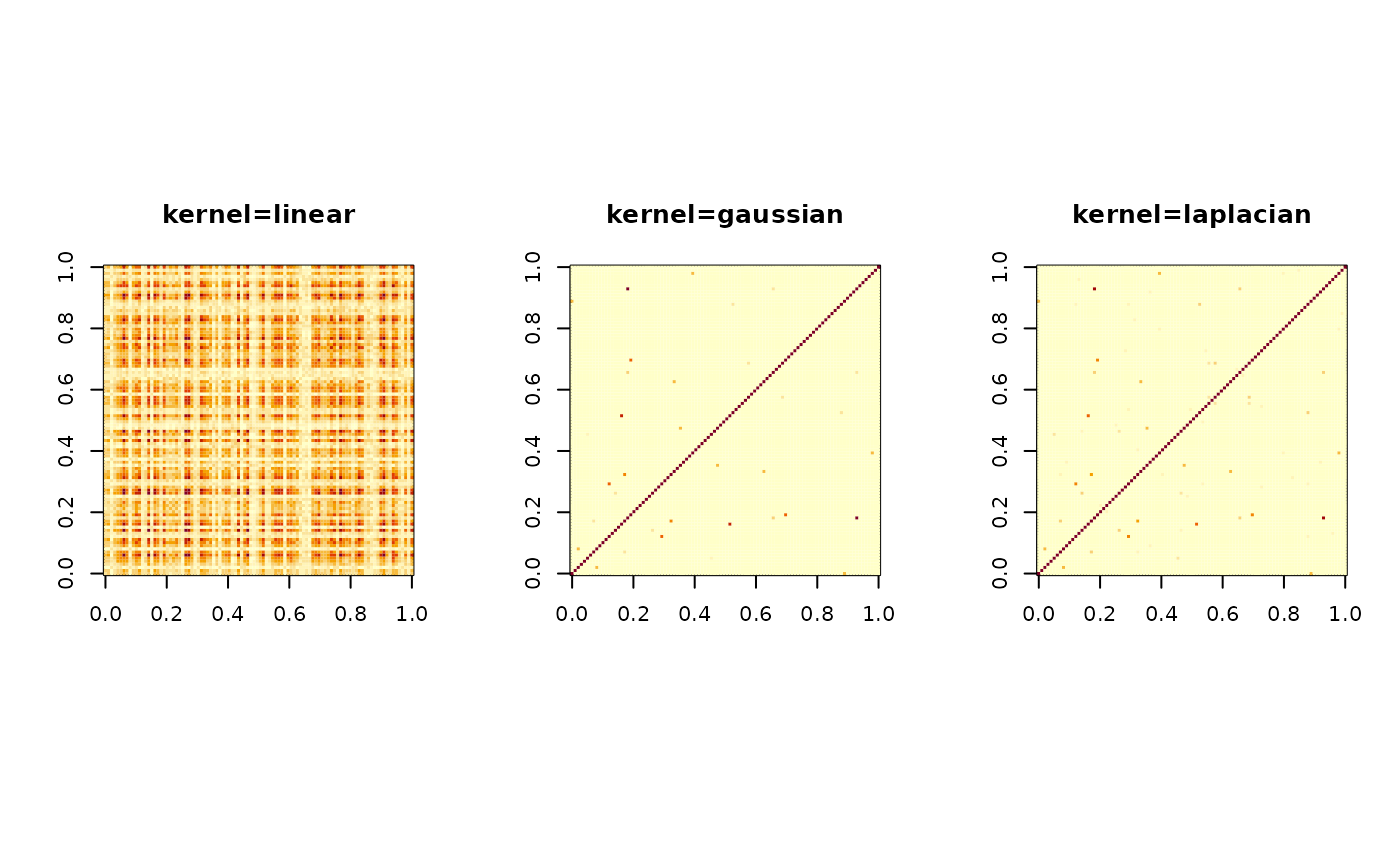
## visualize
opar <- par(no.readonly=TRUE)
par(mfrow=c(1,3), pty="s")
image(Klin$K, main="kernel=linear")
image(Kgau$K, main="kernel=gaussian")
image(Klap$K, main="kernel=laplacian")
 par(opar)
# }
par(opar)
# }